 When presented with a threatened population in need of conservation, the simplest and most basic question a manager can ask is “how big is it?” Unfortunately, this is one of the most challenging questions to answer. Determining the number of individuals in a population is fundamental to effective management. Small, concentrated populations can be destroyed in a single sweep, while large, broadly distributed populations require more resources and complex management involving many stakeholders.
A population that is easy to sample is rare. Animals move – sometimes over enormous distances. Habitats are difficult or impossible to access. Entire popualtions may be adept at avoiding capture. For most populations, it is impossible to count every individual. In marine ecosystems populations can span the entire globe, and the cost of mounting an expedition to systematically sample all members is huge. In order to get accurate estimates of the number of individuals, ecologists have had to devise statistical techniques to estimate the size of a population.
Census size (N) is the total number of living individuals in a population and is traditionally estimated through mark/recapture surveys. The basic method behind mark/recapture is:
- Capture a sub-sample of individuals.
- Mark each individual so they can be identified later. The mark can be a physical tag or the documentation of unique distinguishing traits.
- Release the marked individuals back into the population.
- Capture another sub-sample of individuals, containing both marked and unmarked members.
Since you know exactly how many animals were originally tagged, you can calculate the total number of individuals based on the ratio of marked to unmarked individuals in the second sample. While conceptually simple, this method often requires extensive sampling in order to approach a true estimate of census size. Territoriality may limit the number of individuals in a sample area, populations may be so large that few marked animals are ever recaptured, or life history may make comprehensive sampling impossible.

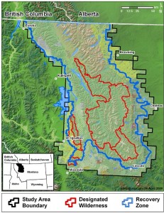
New genetic sampling techniques have made non-invasive mark/recapture studies possible. By sampling feces, hair caught in snares, and other animal leavings, biologists can use DNA as a mark without stressing animals being sampled or modifying their behavior. These non-invasive techniques were implemented in a highly lauded (and politically maligned) Montana Grizzly Bear survey, one of the most thorough and effective population genetics studies to date.
Effective Size and the effect of size
Census size is not the whole story. Not all individuals within a population will survive to reproduce and pass their genes on to the next generation. Reproductive success is far more important than number of individuals in determining the robustness of a population. Effective population size (Ne) is the minimum number of individuals necessary to account for the observed level of genetic diversity in a population. Because it is a genetic estimate, Ne can vary depending on what genes are being examined, the demographic history of the population, recent population expansions or bottlenecks, unequal sex ratios, high variance of reproductive success,non-random mating, multiple paternity, overlapping generations, and the sampling effects of genetic drift (for a basic explanation of drift, please see The Conservation Context in Population Genetics, Part 1).
Another way to think about Ne is that it is an ideal population that will lose genetic variability at the same rate as the census population.
Like Hardy-Weinberg Equilibrium, estimates of Ne are constrained by several assumptions. To estimate Ne, you must assume that the population is free of mutation, migration, and selection, and that the size of the population size is stable across multiple generations.

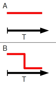
Populations don’t work like that. Take these examples of a stable population and a population undergoing a bottleneck event. In the idealized models, the census size of the stable population remains constant through time, while the population undergoing a bottleneck remains constant, experiences an instantaneous decline, and remains constant at a reduced level.

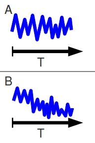
In the real world, populations don’t behave so cleanly. Even a healthy stable population is constantly in a state of flux. The census size of the population changes with each generation, sometimes getting dangerously close to zero and sometimes booming. Even in a bottleneck scenario, the census size varies from year to year. Some of the post-bottleneck years are actually more populous than the pre-bottleneck years, but the general trend is still towards decline.
So how do we calculate effective population size in real world systems?
Variation in time and space
To begin, you need to understand what you’re really measuring. To do this, you need to determine the temporal scale you’re working on and define what genetic phenomena you’re actually measuring.
Contemporary Ne is a measure of effective population size taken between two time points. It is roughly the average size of the population between those two points. In contrast, historic Ne is an average of effective population size over several generations. Historic Ne may come closest to estimating global Ne for the species. If you’re interested in a stable population, the variance effective size (NeV) is the size of an ideal population experiencing drift at the same rate as the census size. Alternatively, if you’re looking at a population that has undergone a bottleneck, the inbreeding effective size (NeI) is the size of a population losing heterozygotes at the same rate as the census size.
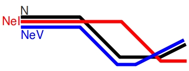
These values respond differently to changes in census size. In a population that has been stable for a long time, both NeV and NeI will be roughly equivalent. As a population enters a bottleneck (which, remember, is not an instantaneous event) NeV will decrease as alleles are randomly removed from the population and the rate of drift accelerates. NeI will lag behind NeV during the bottleneck, because the proportion of heterozygotes to homozygotes will remain roughly constant (assuming the alleles are not linked to the selective pressure cause the bottleneck). Post-bottleneck, as the population returns to Hardy-Weinberg Equilibrium and begins to expand, NeI will fall as the reduced number of alleles become fixed in the population. It will take a long time for NeI to return to pre-bottleneck levels, even if the census size recovers. NeV will rise with increasing census size, but lag behind it.

These effects all depend on a few key assumptions:
- Genetic markers are biparentally inherited.
- The population is sampled at random.
- There is no subdivision of the population.
- There is no immigration.
- There are no overlapping generations.
- The population size is stable!
- There is either no mutation or the mutation rate is known.
Again, population stability continues to confound estimates of effective population size.
Why does variance effective size behave the way it does? Remember that variance effective size is linked to genetic drift. In general, for a population the satisfies the assumptions above, it is much easier to lose alleles that to gain them. Generations with the smallest census size will therefore have a more significant effect on NeV than generations with large census sizes. This means that all contemporary estimates of NeV represent a harmonic mean Ne weighted towards the lowest census size of the population.
Living in the moment
How do you estimate Ne when you don’t have samples from two time points? When estimating effective size from a single point, you’re considering historic, not contemporary effective size. As alleles sort randomly in a population in flux, some alleles may be inherited together as a result of founder effects or drift. This creates the appearance of linkage between the alleles. This non-random association of alleles can be used to estimate NeV from a single sampling event. Linkage disequilibrium should be approached with caution in Conservation Genetics studies as it has been shown to be ineffective when the sample size is small.
An alternative is to determine the effective number of breeding individuals in a population (NeB), which can stand in for Ne but is restricted to systems where breeders can be aggregated and counted.
When dealing with small populations, heterozygote excess can be used to circumvent the issues involved with linkage disequilibrium and can give you an idea of what the population is doing. In a small, but stable population, offspring will generally have more heterozygotes than their parents. A population undergoing a bottleneck will show sign of fixation and have fewer heterozygotes that expected, while a rapidly expanding population of randomly mating individuals with have a excess of heterozygotes.
The classic estimates of effective size based on stepwise mutation and infinite allele models are actually historic estimates of NeI. These are based on the assumptions that heterozygosity is caused by mutation and drift acting in equilibrium, that the mutation model is known, and that mutation rates are the same across all loci.
In contrast, the coalescent allows for a more relaxed estimate of historic NeI based on inferred genealogies. Unlike every other method presented so far, the coalescent does not rely on the assumptions of Hardy-Weinberg Equilibrium. Instead, it constructs inferred genealogies based on current allele distribution to approximate how far back in time different alleles converge, and then use those coalescent events to estimate how many individuals are necessary to achieve that coalescence. While other historic estimators of effective size are essentially forward looking, the coalescent takes an entirely different approach. While the coalescent does allow a relaxed assumption of no migration, it assumes that NeI has been large for a long time, and may not be appropriate for populations in the midst of decline.
Population size is not trivial
The central point to take home from all of this is that determining the size of a population is not a trivial task. Populations fluctuate. Before you can even begin to sample for population size, you need to determine what you really want to know. Are you worried the population is in decline? Do you want to know how large the population has been in the past? Are you concerned with signs of drift, migration, expansion, or selection? Recently or over long stretches of time? What does the current census size mean in light of historic variation in Ne? Historic and contemporary estimate of population size vary. N, Ne, NeV, and NeI are all trying to capture different aspects of a population that is constantly changing. Pay attention to the assumptions. Use multiple, but rational estimates.
Effective population size is really about describing trends and changes in populations. Absolute counts of individuals is reserved for populations on the brink of extinction.
~Southern Fried Scientist
This post is part of the ongoing Crowdsourcing ConGen project. The goal of which is to produce a comprehensive and accessible introduction to Conservation Genetics for managers, conservationists, and interested parties that do not possess a technical background in genetics. Because of this, the focus of this piece is not on how to produce data or calculate each of the values discussed, but to provide the tools to understand and discuss assessments of population size and to be aware of the limitations of each technique.
As always, critical review of both the content and style is not only welcome, but essential for the success of this project. Anyone interested in digging deeper into the concepts presented here should peruse the following papers.
Charlesworth B (2009). Fundamental concepts in genetics: effective population size and patterns of molecular evolution and variation. Nature reviews. Genetics, 10 (3), 195-205 PMID: 19204717
England, P., Cornuet, J., Berthier, P., Tallmon, D., & Luikart, G. (2006). Estimating effective population size from linkage disequilibrium: severe bias in small samples Conservation Genetics, 7 (2), 303-308 DOI: 10.1007/s10592-005-9103-8
Kendall, K., Stetz, J., Boulanger, J., Macleod, A., Paetkau, D., & White, G. (2009). Demography and Genetic Structure of a Recovering Grizzly Bear Population Journal of Wildlife Management, 73 (1), 3-17 DOI: 10.2193/2008-330
Kalinowski, S., & Waples, R. (2002). Relationship of Effective to Census Size in Fluctuating Populations Conservation Biology, 16 (1), 129-136 DOI: 10.1046/j.1523-1739.2002.00134.x
Waples, R. (2005). Genetic estimates of contemporary effective population size: to what time periods do the estimates apply? Molecular Ecology, 14 (11), 3335-3352 DOI: 10.1111/j.1365-294X.2005.02673.x